Creating presence-absence rasters in 2022

Back in 2013 I published a post with a little function for creating presence-absence rasters from point data. I was in the midst of creating ~1000 species distribution models for Australian species and I needed something that I could easily automate in R.

Both R and my approach to working with spatial data have changed a lot in the last nine years, particularly with excellent new packages such as sf and fasterize. This post is a brief update to a new option for creating presence-absence rasters, prompted by a reader’s question.

The steps are essentially the same but I’ve adopted some new packages (sf and fasterize) that make life easier:

1. Create an sf point data set from a dataframe of point locations using st_as_sf.
2. Convert the points to polygons using st_buffer. This step is necessary as fasterize currently doesn’t work with points. For this simple example, I’ve elected to leave my points in WGS84, which means I get a warning that st_buffer doesn’t work properly with lat/long data. I could have used st_transform to convert it to a different projection before using st_buffer.
3. Convert the polygons to a raster¹ using fasterize and then mask out the ocean.

Step 1: Load packages and get the point data

require(biomod2) # for the spatial data
require(dplyr) # for tidy data wrangling
require(sf) # for working with spatial data
require(raster) # for masking rasters
require(fasterize) # for creating the raster


# set select to come from dplyr rather than raster
select <- dplyr::select

# read in a raster of the world
world <- raster(system.file( "external/bioclim/current/bio3.grd",package="biomod2"))

# read in species point data and extract data for foxes
mammals <- read.csv(system.file("external/species/mammals_table.csv", package="biomod2"), 
                    row.names = 1) 

head(mammals)  

X_WGS84  Y_WGS84 ConnochaetesGnou GuloGulo PantheraOnca PteropusGiganteus
1   -94.5 82.00001                0        0            0                 0
2   -91.5 82.00001                0        1            0                 0
3   -88.5 82.00001                0        1            0                 0
4   -85.5 82.00001                0        1            0                 0
5   -82.5 82.00001                0        1            0                 0
6   -79.5 82.00001                0        1            0                 0
  TenrecEcaudatus VulpesVulpes
1               0            0
2               0            0
3               0            0
4               0            0
5               0            0
6               0            0

Step 2: Convert the point data to polygons

# extract fox data from larger dataset and keep only the x and y coordinates
fox_data <- mammals %>% 
  # keep only the spatial data and foxes
  select(X_WGS84,Y_WGS84,VulpesVulpes) %>% 
  # keep only the presence points for foxes
  filter(VulpesVulpes %in% 1) %>% 
  # convert to an sf points object projected in WGS84
  st_as_sf(coords=c("X_WGS84","Y_WGS84"),
           crs = 4326) %>% 
  # convert to an sf polygon object by buffering the points
  st_buffer(1) 

Warning in st_buffer.sfc(st_geometry(x), dist, nQuadSegs, endCapStyle =
endCapStyle, : st_buffer does not correctly buffer longitude/latitude data

head(fox_data)

Simple feature collection with 6 features and 1 field
Geometry type: POLYGON
Dimension:     XY
Bounding box:  xmin: -95.5 ymin: 72.00001 xmax: -75.5 ymax: 74.00001
Geodetic CRS:  WGS 84
  VulpesVulpes                       geometry
1            1 POLYGON ((-93.5 73.00001, -...
2            1 POLYGON ((-87.5 73.00001, -...
3            1 POLYGON ((-84.5 73.00001, -...
4            1 POLYGON ((-81.5 73.00001, -...
5            1 POLYGON ((-78.5 73.00001, -...
6            1 POLYGON ((-75.5 73.00001, -...

Step 3. Create the presence-absence raster

fox_raster <- fasterize(fox_data, world,
                        # select the column to use in the raster
                        field = "VulpesVulpes",
                        # set the value of the background points 
                        background = 0) %>% 
  # only retain values in non-NA cells in the original raster
  mask(world)

Presence (green) – absence (grey) raster of foxes based on the data available in Biomod2

In this plot, the presences (1) are shown in green and the absences (0) in light grey. Now I could have kept the absences in the original dataset and created the raster without using the mask but I wanted to demonstrate what you would need to do if your dataset doesn’t include absence data (which seems to be the most typical scenario).

Pro tip: don’t forget to check that your species point data and raster are in the same projection and that they actually overlap before you get started.

Hopefully this is helpful. But, as always, there are many ways to do things in R and this may not be the most efficient method. I’d be interested to know how else folks are doing this sort of thing.

¹ Note that you need to use a single layer raster for this approach to work as expected. If you have a raster brick or raster stack, then you can either calculate some summary statistics using the fun argument or you can pull out a single layer of the raster brick/stack by using subset(my_raster,layer) or my_raster[[layer]] where layer could be a name or index value.

New paper – Inside or outside: quantifying extrapolation across river networks

It’s been pretty quiet over here for a long time. But I have been busy beavering away at many interesting projects at NIWA, including a project where we developed a new method for identifying when your regression model is starting to make things up (or more technically, extrapolating beyond the bounds of the dataset).

Regression models are used across the environmental sciences to find patterns between a response and its potential predictors. These patterns can be used to predict a response across broad areas or under new environmental conditions. Our paper compares performance of two flexible regression techniques when predicting across a deliberately induced spectrum of interpolation to extrapolation. Various data sets were divided into two geographical, environmental and random groups. Models were trained on one half of the data and tested on the other. The two methods incorporate nonlinear and interacting relationships but suffer from unquantified uncertainty when extrapolating. Random forests always performed better than multivariate adaptive regression splines when interpolating within environmental space, and when extrapolating in geographical space. Random forests models were transferable in geographic space but not to environmental conditions outside the training data. Neither technique was successful when extrapolating across environmental gradients. The paper also describes and tests a new method to calculate degree of extrapolation: a value quantifying interpolation versus extrapolation for each prediction from either regression technique. The method can be used to indicate risk of spurious predictions when predicting at new locations (e.g., nationally) or under new environmental conditions (e.g., climatic change).

Booker, D.J. & A.L. Whitehead. (2018). Inside or outside: quantifying extrapolation across river networks. Water Resources Research. doi:10.1029/2018WR023378 [online]

Santa’s Little Helper – a function for randomly assigning Secret Santa presents

Christmas can be a stressful and expensive time of year, with many gifts to buy for many people. My family have tried to eliminate some of this stress by having a Secret Santa gifting system where we all buy one present for one member of the family on behalf of everybody else, with a cap of $50 per present.

In our family scheme, there are 3 rules:
1. You can’t give a gift to yourself,
2. You can’t give a gift to your partner (we figure that this will happen anyway),
3. You can’t give a gift to someone you gave one to last year.

Somewhere along the line, I’ve become the designated present-assigner. Now I could write names on pieces of paper and put them in a hat but 1) writing out 11 names is tedious, 2) I don’t have a suitable hat and 3) the rules above mean that there are quite often gifting conflicts arise that require the need for a redraw. So I’ve whipped up a little function in R that does the job. (Admittedly it probably would have been faster to use bits of paper but now I’m prepared for next year).

SantasLittleHelper <- function(myFrame,guestList,conflictCols = NULL){
  myTest <- TRUE
  nElves <- 0

  while (myTest == TRUE){
    myOut <- data.frame(gifter = myFrame[,guestList],
                        giftee = sample(myFrame[,guestList],
                                        replace = FALSE,
                                        size=nrow(myFrame))
                        )

    # check that guests haven't drawn themselves
    guestTest<- unlist(lapply(1:nrow(myOut),function(x) {
      myOut$giftee[x] == myFrame[x,guestList]
      }))

    # check for gifting conflicts
    if(!is.null(conflictCols)){

    conflictTest <- unlist(lapply(1:nrow(myOut),function(x) {
      grepl(myOut$giftee[x],myFrame[x,conflictCols])
      }))

    myTest <- any(c(guestTest,conflictTest[!is.na(conflictTest)]))

    } else{
      myTest <- any(guestTest)
    }

    # count the number of iterations needed to avoid conflicts
    nElves <- nElves + 1
  }

  message(paste(nElves,"elves were needed to generate the gift list"))
  return(myOut)
}

SantasLittleHelper takes three arguments: myFrame is a dataframe containing the list of guests to be assigned gifts; GuestList is the character name of the column containing the list of guests; and conflictCols is an optional character vector of column names that identify gifting conflicts that need to be avoided [¹]. The function randomly assigns a giftee to each guest and then checks for conflicts. If conflicts exist, the gifts are reassigned and this continues using a while loop until a suitable solution is found. The function returns a dataframe containing detailing the gifter – giftee combinations, as well as outputting the number of elves (or iterations) needed to generate the list.

To run this for the 2016 Whitehead Family Christmas, I generated a dataframe guests where the column guest lists all of the people coming to Christmas, partner identifies everybody’s significant others and presents2013 lists the assigned giftees from 2013 (the last time we did the Secret Santa thing).

guest	partner	presents2013
John	Fay	Jo
Sue	Simon	Fay
Amy	Hamish	Sue
Jo	Phil	Hamish
Ashley	Naomi	Phil
Naomi	Ashley	John
Phil	Jo	Simon
Hamish	Amy	Naomi
Simon	Sue	Ashley
Fay	John	Amy
Zac	NA	NA

These data are fed into SantasLittleHelper and, bingo, the Whitehead Family Christmas is sorted for another year.

giftList <- SantasLittleHelper(myFrame = guests,
                               guestList = "guest",
                               conflictCols  = c("partner","presents2013")
                               )

27 elves were needed to generate the gift list

gifter	giftee
John	Zac
Sue	Ashley
Amy	Phil
Jo	Amy
Ashley	Fay
Naomi	Sue
Phil	John
Hamish	Jo
Simon	Naomi
Fay	Simon
Zac	Hamish

Hope everyone survives the silly season!

[¹] Technically you could use this feature to rig the outcome to avoid getting a present from Great Aunt Myrtle or Bob from Accounts by adding in an additional conflict column. Use your powers wisely or the ghosts of christmas past may come back to bite you!

Three new papers: urban development, agriculture & skua

What do urban development, agriculture and skua have in common? Superficially very little, except that they feature in three papers that I published in the past few weeks. These papers are the culmination of  research projects I worked on at Landcare Research and the Quantitative & Applied Ecology group at The University of Melbourne and it’s super exciting to see them finally out in print. Many thanks to the teams of co-authors who made these possible.

---

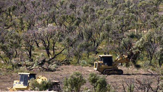
Protecting biodiversity while planning for development

Clever strategic planning can identify land for urban development that minimises habitat clearing and benefits native plants and animals. Picture: WWF-Australia.

As our cities expand due to population growth, development encroaches on the natural habitat of native plants and animals. While developers often have to assess how their new subdivision or industrial park will impact on these populations, this is usually done at the scale of individual developments and often only considers a few species. The consequence of such ad-hoc assessment is that biodiversity can undergo “death by a thousand cuts” where the cumulative impacts of many development projects can be more severe than those predicted by the individual assessments. However, a lack of good tools and guidance has limited  how impact assessments are carried out. We looked at how existing conservation planning tools can use information on the distribution of many species over large areas to identify the potential impacts of a large-scale development plan in Western Australia. We worked closely with government agencies to identify important areas for biodiversity conservation and make minor changes to the development plans that significantly reduced the potential impacts to biodiversity. See our paper for more details on our framework for undertaking strategic environmental assessments.

Whitehead, A., Kujala, H., & Wintle, B. (2016). Dealing with cumulative biodiversity impacts in strategic environmental assessment: A new frontier for conservation planning Conservation Letters DOI: 10.1111/conl.12260

---

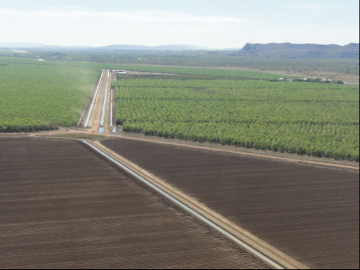
Can biodiversity, carbon and agricultural development coexist in Australia’s northern savannas?

Irrigated agriculture in the Ord River Development. Developing northern Australia will involve trade-offs with biodiversity. (Image credit: Garry D. Cook)

There’s a lot of talk about developing Australia’s north, of doubling the agricultural output of this region and pouring billions of dollars into new infrastructure such as irrigation. But what about the natural values of this region and its potential for carbon storage today and into the future? Can we develop the north and still retain these other values?  We undertook a spatial analysis which found agricultural development could have profound impacts on biodiversity OR a relatively light impact, it all depends on how and where it’s done. If managers and decision makers want northern Australia’s sweeping northern savannas to serve multiple purposes then they need to plan strategically for them. For more information about how such strategic planning could be done, check out our paper and the associated press release.

Morán-Ordóñez, A., Whitehead, A., Luck, G., Cook, G., Maggini, R., Fitzsimons, J., & Wintle, B. (2016). Analysis of trade-offs between biodiversity, carbon farming and agricultural development in Northern Australia reveals the benefits of strategic planning. Conservation Letters DOI: 10.1111/conl.12255

---

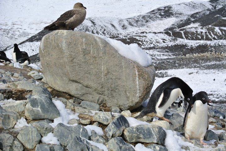
Counting skua by counting penguins

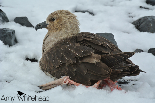
A skua surveying potential lunch options at the Cape Bird Adélie penguin colony.

South polar skua (Stercorarius maccormicki) like to chow down on penguins. So it makes sense that they often nest close to penguin colonies. Over the years, we’ve developed a pretty good understanding of the size of Adélie penguin (Pygoscelis adeliae) colonies around the Ross Sea, Antarctica, so we set out to see if we could estimate the number of skua associated with those colonies.  Detailed surveys of skua at three Adélie penguin colonies on Ross Island confirmed that more penguins (i.e. more lunch) means more skua.  Using this relationship, we predicted how many skua live in the Ross Sea. To find out how many skua live in the Ross Sea and for a more detailed description of the methods, check out our paper online.

Wilson, D., Lyver, P., Greene, T., Whitehead, A., Dugger, K., Karl, B., Barringer, J., McGarry, R., Pollard, A., & Ainley, D. (2016). South Polar Skua breeding populations in the Ross Sea assessed from demonstrated relationship with Adélie Penguin numbers. Polar Biology. DOI: 10.1007/s00300-016-1980-4

Extracting raster data using a shapefile

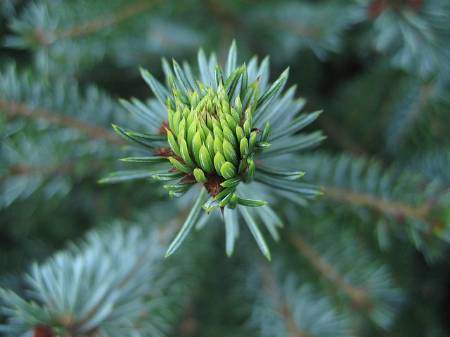
I recently had an email from a PhD student in Austria who had a raster showing the distribution of Douglas Fir in Europe and wanted to know what proportion of each European country was covered in this species. They had a raster with presence (1) and absence (0) of Douglas-fir in Europe and wanted to calculate the number of cells with 1 and 0 within each country of the Europe. I’ve put together a dummy example below which shows how to R script to extract the number of raster cells in each country that meet a certain condition.

Douglas Fir (source: Pixabay)

Essentially the script works through the following steps:

1. Loads the relevant shapefile and raster datasets.
2. Identifies all of the countries within the shapefile.
3. Within a loop, masks the presence-absence raster by each country and counts the number of cells that meet the required condition.

Goodbye Melbourne, hello (insert adventure here)

As I shut down my laptop for the last time and handed back my office keys a couple of months ago, it was hard to believe that two and a half years earlier, I had packed up my life in shaky Christchurch and moved to Melbourne to start a one year contract with the Quantitative & Applied Ecology group. Like most of the positions in my random career trajectory, I came to Melbourne by (happy) accident. I had applied for a position elsewhere in Australia and didn’t get it. But the guy who interviewed me mentioned this other guy in Melbourne who might have a position. We had a brief chat over the phone which essentially covered “Do you know how to use MaxEnt & Zonation?” & “When can you start?” to which I replied “Sure” & “Soon”.  A month later, I moved to Melbourne to start work with Brendan Wintle. The work has been interesting and varied, although largely concentrating on developing species distribution models to use in real-life conservation planning exercises aimed at informing Strategic Assessments in several regions of Australia. This has included lots of modelling, over a hundred meetings with stakeholders and lots and lots of squinting at maps and swearing at R code.  I also worked with some amazing colleagues, now amazing friends, and generally had a great time in Melbourne. Amazingly, in the two years or so since I started this blog, I have never written about the research I’ve been doing in Melbourne. The QAECO blog has a couple of posts about incorporating social values into conservation planning and some poetry that I wrote about a colleague but, at some point, I should probably remedy that.  But for now, here’s a story about my next adventure….

Not long after I bid my fond farewell to the folks of QAECO, I flew west to Perth to be reunited with my partner of seven years. It had been 4.5 years since we had lived in the same city, so it seemed like it was probably time we did something about that. Since then, I’ve been enjoying the Perth sunshine, finishing up a few work projects and playing travel agent. For we are off on a bike ride.

A big bike ride. Approximately 4,600 km of backcountry bikepacking along the Rocky Mountains from Jasper in Canada to Antelope Wells on the Mexican border. It’s going to be a great adventure and utterly terrifying all at the same time.

What happens when we get back in November is totally up in the air. While a (tiny) part of me feels that I should be worried about not having a plan (particularly an academic plan) for when we get back. But it is actually quite liberating to just have the open road and endless possibilities ahead.

Needless to say, not much will be happening in this little corner of the web in the next few months but you’ll be able to follow our progress (and tales of bear encounters and other fun stories) at ridingtherockyroad.wordpress.com

Nigel Latta (& me) in Antarctica (on the telly)

Last season, when I was in Antarctica, we had a visit from Nigel Latta, a criminal psychologist turned comedic documentary-maker who makes humorous shows about serious subjects. He was sent to Scott Base, Antarctica to live among the scientists and to discover what life on the Ice is really like and whether it holds the key to our futures. The first episode airs on March 4th at 8:30pm on TV One (in NZ only) and promises to be an entertaining ride.

Filming with Nigel and his team was one of the more entertaining media experiences I’ve had – we defused bombs in a tent, counted (& recounted & recounted & recounted & ….) a constantly moving mass of penguin chicks by trying to name them all, discussed the parenting abilities of penguins and their monogamous (or lack thereof) relationships. I watched (with delight) as Nigel got shat on by a South Polar skua and attacked by angry penguins, we restaged Shackelton’s famous dinner photo and generally had a rollocking good time. I look forward to seeing his thoughts of life On Thin Ice*.

If you miss it (& happen to live in NZ), you should be able to watch it OnDemand.

* Not that I will actually be able to watch it, what with not being in NZ and the restrictions of TV OnDemand….but I’d love to know what you think of it.

Copying files with R

Following on from my recent experience with deleting files using R, I found myself needing to copy a large number of raster files from a folder on my computer to a USB drive so that I could post them to a colleague (yes, snail mail – how old and antiquated!).  While this is not typically a difficult task to do manually, I didn’t want to copy all of the files within the folder and there was no way to sort the folder in a sensible manner that meant I could select out the files that I wanted without individually clicking on all 723 files (out of ~4,300) and copying them over.  Not only would this have been incredibly tedious(!), it’s highly likely that I would have made a mistake and missed something important or copied over files that they didn’t need. So enter my foray into copying files using R.

A day in the life of a penguin wrangler

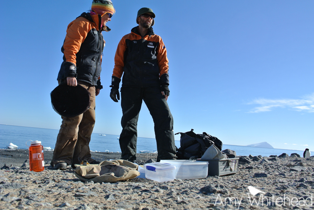
By now you’ve probably figured out that I have something to do with penguins and occasionally disappear for months on end into the wilds of Antarctica. I often get asked what we actually do all day when we’re out in the field but my usual response – “oh, you know, count penguins and stuff” – isn’t really that satisfactory. So I’ve tried to document a typical day in the field at Cape Bird…

08:00¹ Bleep bleep bleep. The alarm goes off and I yank on the piece of string to remove the tightly wedged piece of cardboard in the window and let the daylight stream in. One of the problems of 24 hours of daylight is that it’s hard to block the light out. However, we’ve managed it to overcome that problem so well that we now struggle to wake up because there are no daylight cues to indicate that it’s morning. Hence the string. Eventually dragging myself out of bed, I stumble blindly out to the kitchen and get the coffee pot going. The boys are busy burning the toast while trying to identify a seal drifting past on the sea ice. At first glance, it looked like it might be a leopard seal but, on closer inspection through the binoculars, it turns out to be a weddell seal. They’re pretty common in this neck of the woods, so attention quickly turns back to rescuing breakfast. Then there’s a quick discussion about the plan for the day, which quickly digresses into some random conversation totally off topic!

10:00 We start to layer on the gear in preparation for going outside. It’s not a particularly cold day outside (maybe hovering just below 0°C), so no need to go overboard with the layers. Just a pair of polar fleece trousers, insulated overalls, merino t-shirt, merino longsleeved top, fleece sweater, primaloft jacket and windstopper jacket, topped off with a fleece-lined woollen hat, a neck buff, sunglasses and a pair of possum-merino gloves. Oh, plus a pair of thick woollen socks and insulated boots. It takes a while to get ready! Then it’s outside to start the day’s work.

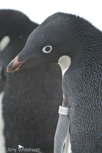
Peter heads off to start bandsearching – walking the edge of the subcolonies and looking for birds with flipper bands. Once located, he’ll record the band number and the bird is up to. This is usually a straightforward process but there is always someone who flaps their flippers or turns so that you can’t read the band. This usually turns into a frustrating game where you and the penguin dance around each other for five minutes (or more!) until eventually you manage to outwit the bird. Once is tolerable but when you’re doing this for 8 hours or more a day, it can get pretty tedious.  On the other hand, spending this much time walking around the colony means you get to see a lot of interesting things and take a lot of pictures.

Hamish & I head down the hill to the weighbridge colony. This small subcolony of approximately 200 nests is surrounded by a mesh fence, with the only access point into the colony across a bridge. This bridge hides a set of scales that weigh birds as they cross, as well as recording whether they coming or going. Every couple of days we download the data from the weighbridge and record the status of the marked nests – which adults are present and how many eggs or chicks they have – as well as the total number of adults and chicks in the subcolony. This information is used to work out some pretty interesting information about how long adults are out at sea and how much food they bring back for their chicks.  It also lets us compare how the colony is doing from year to year.

11:00 Next we head off to count adults and chicks at two more reference colonies. Unlike the weighbridge colony, these subcolonies are not surrounded by a fence. We monitor 30 marked nests in these colonies from early November when the eggs are laid until the chicks creche in mid January. While we’re walking between colonies, we find a freshly dead chick that has just been killed by a skua. Penguin colonies are filled with death and destruction and it can take a bit of getting used to. But it can also offer some unique opportunities. All dead chicks in reasonable condition (i.e. they are still whole and not super stinky) are weighed, measured and then dissected. Looking at the stomach contents gives us some idea about what’s happening out at sea. This chick has been fed mostly krill but the grey mush suggests that adults are also starting to bring in silverfish. This tends to happen later in the season when the chicks are about three weeks old.

 

12:00 Chick counting done for the moment, it’s off to do some actual penguin wrangling. Since we arrived in mid December we’ve been catching banded adults with chicks and attaching small devices called accelerometers. These collect information about a bird’s foraging behaviour: how long they spend out at sea on one foraging trip, how often and how deep they dive, and the types of movements they are making while under the water. This morning’s task is to look for birds with accelerometers that that have returned from sea. Foraging trips typically last anywhere from 2 – 8 days, depending on the conditions out to sea. This year they seem to be at the longer end of the scale, suggesting that it’s taking longer for birds to find enough food to feed themselves and their chicks.

We aim to recatch birds when they have returned to their nests and are happily brooding their chicks. This is for three reasons:
1) it hopefully gives the adult time to feed their chick(s) before we turn up to disturb them; 2) it’s by far the easiest way to find them (imagine looking for a penguin with a small black device attached to its black back amongst ~40,000 other black-backed penguins!); and 3) adults are much easier to catch if they are sitting on a nest. Grabbing a penguin off a nest is much easier than you might expect – you simply weave your way through the surrounding nests (getting thoroughly pecked and beaten by the neighbours in the process) and pick them up. A second person collects the chick(s) and leaves a cover over the nest to stop the neighbours stealing all the rocks while you’re away. Then it’s onto the business of taking a blood sample, removing the accelerometer and taking a range of measurements such as weight and flipper length. Once the adult has been processed, we weigh and measure the chicks before marking them with a temporary plastic tag. These individually-numbered tags mean that we can follow the growth and survival of these chicks throughout the season. Once we’re done, we release the adult and the chicks back on the nest. The whole process takes less than 20 minutes for each bird and is relatively stress-free for both penguin and wrangler. This morning we manage to retrieve three of the ten accelerometers we have out, which is a pretty good haul.

 

14:00 Blood samples and accelerometers in hand, it’s time to head back to the hut and process the samples. Vials of blood are loaded into the centrifuge and sent spinning merrily on their way, slides are fixed in alcohol, feather samples are stored away under the bench and the first accelerometer is plugged into the computer to download. It must be time for lunch! This year we’ve become masters of the scone and today’s lunch includes a healthy dose of the chocolate and date variety, with a side of toasted cheese sandwich and some dried apple slices.

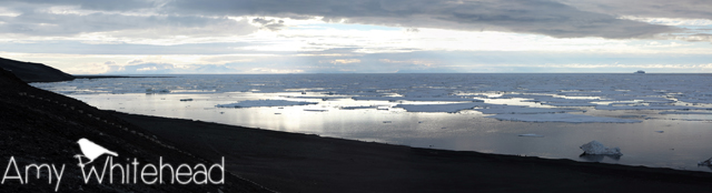
It can take up to 40 mins to download the data from each accelerometer. Given that we have three to do today, we have plenty of time to do our daily mammal survey. This involves staring out the window for an hour every day, scanning the beach and water for mammals. We often see Weddell seals on the beach and some days will be treated to a Antarctic minke whale or a pod of orca swimming past. Alas, today is not one of those days and it’s a very long hour staring out the window with binoculars without seeing a single mammal. At least the view isn’t too shabby.

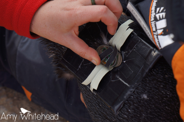
16:30 Blood processed, accelerometers downloaded, lunch eaten and the lack of mammals surveyed, it’s time to head back outside to finish the rest of the day’s fieldwork. We hope to put the three accelerometers that we retrieved this morning back out on some new birds. We have a list of target nests with banded birds of known ages, so it’s simply a matter of walking around and checking those nests until we find somebody at home. Once we’ve located a victim customer, it’s a matter of grabbing the bird and its chicks off the nest and attaching the accelerometer. We do this using thin strips of tape that are layered under the feathers, a technique that is robust enough to stay on for up to three foraging trips. A nice, non-wriggly bird will take about 5-6 minutes to process and return to the nest. A wriggly bird may take a bit longer and will likely result in some strong words from the handler and the tape sticker! Oh how we hate the wriggly birds!

18:00 Three accelerometers deployed, it’s time to go and count some more penguins. As the season progresses, the number of adults at a subcolony decreases as the chicks are left to creche. This leaves the chicks particularly vulnerable to skua predation. We have some small subcolonies of penguins just below the hut that are quite isolated and surrounded by skua nests. These colonies drop in size quite dramatically as chicks start to disappear into the mouths of skuas. [skua swallowing chick photo] The skua effect can be so severe that the smallest of these colonies rarely manages to fledge any chicks. Every couple of days we count the number of adults and chicks to document the skua-induced declines. Today everyone seems to be well and accounted for but there are six hungry skua stalking the edge of the colony, so I suspect that the next counts will be somewhat lower.

18:30 Heading back up to the hut, we dump our packs and pick up some shovels and a wheelbarrow, and head over to the snowbank. Our hut has no plumbing system, so we have to collect snow to melt for water. A couple of times a week, we shovel snow into the wheelbarrow and dump it in a large container in the hut where it slowly melts. We also have to carry all our waste water (including pee) in buckets down to the sea. As such, washing is an event that is much less regular than would be socially acceptable in the real world! Luckily, we all smell equally of penguin.

 

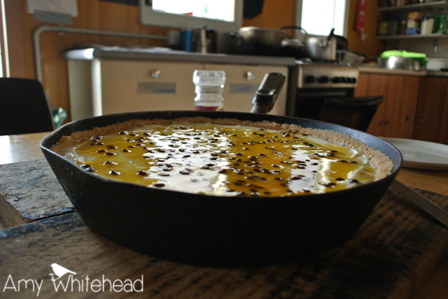
20:00 “Scott Base, Scott Base, this is Cape Bird”. Every night we check in with Antarctica NZ at Scott Base on the VHF radio to let them know we’re okay and haven’t been eaten by skua or drifted away in a boat². It’s our only opportunity to talk to someone outside of our group of three, hear some news from the outside world and get a weather report. Then it’s time for dinner – usually some sort of stirfry/pasta/curry dish. Today it’s a variation on lamb stirfry, followed by a special treat – passionfruit cheesecake! As far as field food goes, we have it pretty good out at Cape Bird. We have a freezer, so we can have frozen meat and vegetables, and there is a large well-stocked pantry with most of the things you need. Like most field huts though, Cape Bird is the place the food goes to die and expiry dates are treated more as a game (“Guess how many years since tonight’s dinner ingredients expired!”³) than a guideline for edibility. And you definitely start to crave fresh food – what we wouldn’t give for a simple salad.

21:00 Fed, watered and dishes washed, we all sit down at our computers and enter the day’s data, download photos, and work out a plan for tomorrow. This year Peter is trialling a new approach to data entry by entering it directly into a tablet in the field. It seems to be working well and saves having to enter up to 14 pages of data at the end of the day but there is still room for improvement. I spend some time in the lab sorting out the bleeding kit; finding more needles, pre-labelling sample bags.

00:00 How did it get to be this late already?! It’s hard to keep track of time when it never gets dark outside and we often find ourselves working much later than we intended. The light at this time of day is often stunning and it’s tempting to head back outside to take pictures. Tonight we set up the timelapse camera to try and capture the moving sea. Then it’s time to wedge the cardboard back in the window and drift off to sleep, counting penguins…

 

¹ This hour of rising may be somewhat optimistic and is purely here for the benefit of my boss (who I’m hoping doesn’t read footnotes!). Even this is much later than the season when he was there but that’s what happens when you leave me in charge!

² This happened to a group of researchers at Cape Bird in the 1970s. It took five days before they were rescued. Needless to say, we are no longer allowed boats!

³ I think 2004 was the oldest expiry date encountered this year, although there were a couple of items that I think actually pre-dated expiry dates!

Converting shapefiles to rasters in R

I’ve been doing a lot of analyses recently that need rasters representing features in the landscape. In most cases, these data have been supplied as shapefiles, so I needed to quickly extract parts of a shapefile dataset and convert them to a raster in a standardised format. Preferably with as little repetitive coding as possible. So I created a simple and relatively flexible function to do the job for me.

The function requires two main input files: the shapefile (shp) that you want to convert and a raster that represents the background area (mask.raster), with your desired extent and resolution. The value of the background raster should be set to a constant value that will represent the absence of the data in the shapefile (I typically use zero).

The function steps through the following:

1. Optional: If shp is not in the same projection as the mask.raster, set the current projection (proj.from) and then transform the shapefile to the new projection (proj.to) using transform=TRUE.
2. Convert shp to a raster based on the specifications of mask.raster (i.e. same extent and resolution).
3. Set the value of the cells of the raster that represent the polygon to the desired value.
4. Merge the raster with mask.raster, so that the background values are equal to the value of mask.raster.
5. Export as a tiff file in the working directory with the label specified in the function call.
6. If desired, plot the new raster using map=TRUE.
7. Return as an object in the global R environment.

The function is relatively quick, although is somewhat dependant on how complicated your shapefile is. The more individual polygons that need to filtered through and extracted, the longer it will take.